Single-Image 3D Gaussian Splatting in One Forward Pass

In my previous blog, we tackled single-view 3D reconstruction by optimizing a NeRF from a learned initialization. Meta-learning gave us a category-aware starting point, so adaptation only needed a few gradient steps.

But the optimization loop was still there.

This post takes the other route: feedforward 3D Gaussian Splatting. Instead of optimizing 3D parameters per scene, we train a network that maps an image to a full 3DGS representation in a single forward pass. No test-time optimization, no inner loop, no hours of fitting — one image in, a complete set of 3D Gaussians out.

The idea comes from the paper:

Splatter Image: Ultra-Fast Single-View 3D Reconstruction — Szymanowicz, Rupprecht, Vedaldi (CVPR 2024)

The implementation below is a compact PyTorch version of that idea, applied to single-view object reconstruction on the ShapeNet dataset. This is also the first post in a short series on feedforward 3DGS, so we will be revisiting and extending the method in upcoming posts.

What is feedforward 3D Gaussian Splatting?

Standard 3D Gaussian Splatting fits a set of Gaussians to a scene by optimization: you start from a sparse point cloud, define a photometric loss against multi-view images, and run gradient descent for thousands of iterations. The result is excellent quality — at the cost of minutes to hours per scene.

Feedforward 3DGS asks the opposite question:

Can we predict the Gaussians directly with a neural network, instead of optimizing them?

If a network has seen enough scenes from the same distribution, it can learn the priors that optimization usually has to rediscover from scratch. The network outputs a 3DGS representation in one forward pass, and we render with the standard differentiable rasterizer.

Splatter Image is the simplest, most elegant instance of this idea: one Gaussian per input pixel, predicted by a UNet.

Why this matters

3D Gaussian Splatting is fast at rendering, but slow at fitting. Optimizing a 3DGS scene from images can take minutes to hours. Feedforward 3DGS replaces that loop with a single forward pass.

The Splatter Image trick:

What if a UNet could predict 3DGS parameters directly from an image, the way it predicts a depth map?

Concretely: each pixel of the input image becomes one 3D Gaussian. A UNet that takes a [3, H, W] image and outputs a [15, H, W] feature map encodes all the parameters of H × W Gaussians at once.

That gives us:

• one forward pass instead of an optimization loop
• a learned category-level prior baked into the network weights
• a continuous 3D representation that works with the standard Gaussian rasterizer

Conceptually, this is the opposite of last week's post: predict the representation rather than optimize it.

1. The big picture

The pipeline has three stages:

1. A UNet predicts raw Gaussian parameters. Input: source image. Output: a 15-channel feature map, one Gaussian per input pixel.
2. A decoder turns those raw outputs into valid Gaussians. Depths get unprojected along camera rays, scales are exponentiated, quaternions are normalized, and a covariance matrix is assembled.
3. A differentiable rasterizer renders those Gaussians from a target view. We compare the rendering to the ground-truth target image with MSE.

Training is supervised on novel views. For each scene, we sample two views — one source and one target. The model only ever sees the source. Its predicted Gaussians are rendered from the target camera and compared to the target image.

2. The 15 channels per pixel

Each of the 15 output channels has a fixed meaning:

• 1 channel — opacity (raw, passed straight to the renderer)
• 3 channels — XYZ offset from the camera ray
• 1 channel — depth along the ray (raw, sigmoid-scaled later)
• 3 channels — scale, in log-space
• 4 channels — quaternion (xyzw)
• 3 channels — RGB color (raw, sigmoid-scaled later)

The model never directly outputs a 3D position. Instead, it outputs a depth along the ray plus a small offset. The position of each Gaussian is then origin + u · depth + delta, where u is the normalized pixel ray. This conditioning on the source camera makes training significantly more stable — the network only has to learn local geometry instead of arbitrary world-space coordinates.

3. Decoding the Gaussian positions

The decoder takes the raw [1, 15, H, W] UNet output and produces world-space Gaussian parameters. Let's start with the means (the 3D centers).

def decode_gaussians(raw, source_c2w, fx, fy, cx, cy, znear, zfar, opacity_threshold=0.0):

    device = raw.device
    dtype = raw.dtype
    _, _, H, W = raw.shape

    opacity_raw = raw[:, 0:1]
    delta       = raw[:, 1:4]
    depth_raw   = raw[:, 4:5]
    scale_raw   = raw[:, 5:8]
    quat_raw    = raw[:, 8:12]
    color_raw   = raw[:, 12:15]

    depth = (zfar - znear) * torch.sigmoid(depth_raw.clamp(-10, 10)) + znear

    u = build_pixel_grid_from_intrinsics(H, W, fx, fy, cx, cy, device, dtype).unsqueeze(0)

    Rcw = source_c2w[:3, :3]
    tcw = source_c2w[:3, 3]
    Rwc = Rcw.t()
    origin_cam = (Rwc @ (-tcw)).view(1, 3, 1, 1)

    mean_cam = torch.empty((1, 3, H, W), device=device, dtype=dtype)
    mean_cam[:, 0:1] = origin_cam[:, 0:1] + u[:, 0:1] * depth + delta[:, 0:1]
    mean_cam[:, 1:2] = origin_cam[:, 1:2] + u[:, 1:2] * depth + delta[:, 1:2]
    mean_cam[:, 2:3] = origin_cam[:, 2:3] + depth + delta[:, 2:3]

Three things happen here:

• Depth. The raw depth output goes through a sigmoid and is mapped into [znear, zfar]. This bounds the predicted depths to the scene's expected range.
• Pixel ray. build_pixel_grid_from_intrinsics returns the per-pixel ray direction in camera coordinates: u = (x + 0.5 - cx) / fx, v = (y + 0.5 - cy) / fy, 1. Multiplying by depth gives a 3D point along that ray.
• Offset. The raw delta adds a small XYZ correction. This lets the network move a Gaussian slightly off its ray when geometry doesn't lie exactly on it.

I'm computing means in camera coordinates here — the world-space transformation comes next.

4. Decoding scale, rotation, and covariance

Each 3D Gaussian needs a covariance matrix Σ. The standard 3DGS parameterization writes it as Σ = R S² Rᵀ, where R is a rotation matrix built from a quaternion and S is a diagonal scale matrix.

    color = torch.sigmoid(color_raw)
    quat_xyzw = torch.nn.functional.normalize(quat_raw, dim=1, eps=1e-6)

    pos_cam            = mean_cam[0].permute(1, 2, 0).reshape(-1, 3)
    opacity_raw_flat   = opacity_raw[0].reshape(-1)
    scale_raw_flat     = scale_raw[0].permute(1, 2, 0).reshape(-1, 3)
    quat_flat          = quat_xyzw[0].permute(1, 2, 0).reshape(-1, 4)
    color_flat         = color[0].permute(1, 2, 0).reshape(-1, 3)

    pos_world   = (Rcw @ pos_cam.t()).t() + tcw.unsqueeze(0)
    scales      = torch.exp(scale_raw_flat.clamp(-10.0, 3.0)).clamp_min(1e-6)
    R_local     = quat_xyzw_to_rotmat(quat_flat)
    S           = torch.diag_embed(scales)
    sigma_cam   = R_local @ S @ S @ R_local.transpose(1, 2)
    sigma_world = Rcw.unsqueeze(0) @ sigma_cam @ Rcw.t().unsqueeze(0)

    return pos_world, color_flat, opacity_raw_flat, sigma_world

A few things worth pointing out:

• Scales are exponentiated because the network outputs them in log-space. This guarantees positivity without needing a clamp.
• Quaternions are normalized to lie on the unit sphere. Without this, a small magnitude shift would change the rotation.
• Σ is computed in camera space, then transformed to world space with Σ_world = R_cw Σ_cam R_cwᵀ. This is consistent with the way positions are computed (in camera coordinates first), and lets the network learn local shape independently of scene-level pose.

The output is the canonical 3DGS quintuple: position, color, opacity, covariance — one per pixel.

5. Output head initialization

There is a quietly critical piece in this implementation: how the final output head of the UNet is initialized.

def init_output_head(model, znear=0.8, zfar=1.8, *, opacity_bias=-3.5, depth0=1.2,
                     scale_bias=0.02, opacity_gain=1.0, xyz_gain=0.1, depth_gain=1.0,
                     scale_gain=0.1, quat_gain=1.0, rgb_gain=5.0):

    def inv_sigmoid_scalar(y, eps=1e-6):
        y = max(eps, min(1.0 - eps, float(y)))
        return math.log(y / (1.0 - y))

    with torch.no_grad():
        weight = model.head.weight
        bias = model.head.bias
        weight.zero_()
        bias.zero_()

        depth01 = (depth0 - znear) / (zfar - znear)
        depth_bias = inv_sigmoid_scalar(depth01)

        torch.nn.init.xavier_uniform_(weight[0],     gain=opacity_gain)
        torch.nn.init.constant_(bias[0],             opacity_bias)
        torch.nn.init.xavier_uniform_(weight[1:4],   gain=xyz_gain)
        torch.nn.init.xavier_uniform_(weight[4],     gain=depth_gain)
        torch.nn.init.constant_(bias[4],             depth_bias)
        torch.nn.init.xavier_uniform_(weight[5:8],   gain=scale_gain)
        torch.nn.init.constant_(bias[5:8],           math.log(scale_bias))
        torch.nn.init.xavier_uniform_(weight[8:12],  gain=quat_gain)
        torch.nn.init.constant_(bias[11],            1.0)
        torch.nn.init.xavier_uniform_(weight[12:15], gain=rgb_gain)

Without this step, the network produces nonsense Gaussians at iteration zero and training is unstable. With it, the very first forward pass already produces something sensible.

What each line buys us:

• Opacity bias = -3.5. After sigmoid, this is around 0.03 — Gaussians start nearly transparent. Training has to actively push opacity up where the object exists, which is much more stable than starting opaque everywhere.
• Depth bias. We pick depth0 = 1.2 (middle of the scene volume) and invert the sigmoid to get the corresponding pre-activation. At init, every Gaussian sits roughly in the middle of the depth range.
• Scale bias = log(0.02). Small Gaussians at init avoid a "blob" pattern that would dominate the rendering and confuse early gradients.
• Quaternion bias = (0, 0, 0, 1). Identity rotation. Setting only bias[11] = 1 puts the unit quaternion in canonical position.
• RGB and small gains everywhere else. Modest Xavier init keeps the network's first predictions close to a uniform gray scene.

If you remember one thing from this post, remember this: reasonable parameterization is half the battle in feed-forward 3D models. A clean output head turns a divergent loss into one that descends from step one.

6. The dataset

We use the NMR (Neural Mesh Renderer) cars dataset, with multi-view renderings and known camera matrices.

class NMRDataset(Dataset):
    def __init__(self, data_path, json_path, train=True, n_views=24, H=64, W=64):
        self.data_path = data_path
        self.n_views = n_views
        self.H = H
        self.W = W

        with open(json_path, "r") as f:
            split = json.load(f)

        self.scenes = [
            os.path.join(data_path, f) for f in sorted(split["train" if train else "test"])]

        gt_pixels, c2ws, intrinsics = [], [], []
        for scene_path in tqdm(self.scenes, desc="loading scenes"):
            cam_data = np.load(os.path.join(scene_path, "cameras.npz"))

            scene_gt_pixels   = torch.zeros((n_views, H, W, 3), dtype=torch.float32)
            scene_c2ws        = torch.zeros((n_views, 4, 4),    dtype=torch.float32)
            scene_intrinsics  = torch.zeros((n_views, 4, 4),    dtype=torch.float32)

            for view_idx in range(n_views):
                img = np.array(Image.open(
                    os.path.join(scene_path, "image", f"{view_idx:04d}.png")).convert("RGB"))
                c2w = cam_data[f"world_mat_inv_{view_idx}"]
                K   = cam_data[f"camera_mat_{view_idx}"]

                scene_gt_pixels[view_idx]  = torch.from_numpy(img).float() / 255.0
                scene_c2ws[view_idx]       = torch.from_numpy(c2w).float()
                scene_intrinsics[view_idx] = torch.from_numpy(K).float()

            gt_pixels.append(scene_gt_pixels)
            c2ws.append(scene_c2ws)
            intrinsics.append(scene_intrinsics)

        self.gt_pixels  = torch.stack(gt_pixels,  dim=0)  # [B, N, H, W, 3]
        self.c2ws       = torch.stack(c2ws,       dim=0)  # [B, N, 4, 4]
        self.intrinsics = torch.stack(intrinsics, dim=0)  # [B, N, 4, 4]

Each scene has 24 views, each with image + camera-to-world matrix + intrinsics. Everything is pre-loaded into tensors, so training is I/O-free.

The __getitem__ method is where the source/target sampling happens. For each batch element, we pick one source view (the input to the model) and a different target view (the supervision signal):

    def __getitem__(self, scene_idx):
        scene_imgs  = self.gt_pixels[scene_idx]
        scene_c2ws  = self.c2ws[scene_idx]
        scene_intr  = self.intrinsics[scene_idx]

        src_idx, tgt_idx = sample_source_target_indices(self.n_views)
        return {"src_img":      scene_imgs[src_idx].permute(2, 0, 1),
                "tgt_img":      scene_imgs[tgt_idx].permute(2, 0, 1),
                "source_c2w":   scene_c2ws[src_idx],
                "target_c2w":   scene_c2ws[tgt_idx],
                "source_cam":   scene_intr[src_idx],
                "target_cam":   scene_intr[tgt_idx],
                "meta":         torch.tensor([scene_idx, src_idx, tgt_idx], dtype=torch.long)}


def sample_source_target_indices(n_views):
    src_idx = random.randrange(n_views)
    tgt_idx = random.randrange(n_views - 1)
    if tgt_idx >= src_idx:
        tgt_idx += 1
    return src_idx, tgt_idx

The sample_source_target_indices trick guarantees src_idx ≠ tgt_idx without a rejection loop: pick the target from n_views - 1 slots, then shift it past the source if needed.

7. Training: predict, render, supervise

The training loop is short.

for step in tqdm(range(1, 800_001)):
    try:
        batch = next(train_iter)
    except StopIteration:
        train_iter = iter(train_loader)
        batch = next(train_iter)

    batch_src_imgs    = batch["src_img"].to(device, non_blocking=True)
    batch_tgt_imgs    = batch["tgt_img"].to(device, non_blocking=True)
    batch_source_c2w  = batch["source_c2w"].to(device, non_blocking=True)
    batch_target_c2w  = batch["target_c2w"].to(device, non_blocking=True)
    batch_source_cam  = batch["source_cam"].to(device, non_blocking=True)
    batch_target_cam  = batch["target_cam"].to(device, non_blocking=True)

    optimizer.zero_grad(set_to_none=True)
    raw_batch = model(batch_src_imgs)  # [B, 15, H, W]

    batch_loss = 0.0
    for b in range(batch_size):
        fx_src, fy_src, cx_src, cy_src = intrinsics_to_fxfycxcy(batch_source_cam[b], H, W)
        fx_t,   fy_t,   cx_t,   cy_t   = intrinsics_to_fxfycxcy(batch_target_cam[b], H, W)

        raw_b = raw_batch[b:b + 1]
        pos, color, opacity_raw, sigma = decode_gaussians(
            raw=raw_b, source_c2w=batch_source_c2w[b], fx=fx_src, fy=fy_src, cx=cx_src,
            cy=cy_src, znear=znear, zfar=zfar, opacity_threshold=0.0)

        pred = render(pos=pos, color=color, opacity_raw=opacity_raw, sigma=sigma,
                      c2w=batch_target_c2w[b], H=H, W=W, fx=fx_t, fy=fy_t, cx=cx_t,
                      cy=cy_t).permute(2, 0, 1).unsqueeze(0)

        tgt = batch_tgt_imgs[b:b + 1]
        loss_b = torch.nn.functional.mse_loss(pred, tgt)
        batch_loss = batch_loss + loss_b

    batch_loss = batch_loss / batch_size
    batch_loss.backward()
    optimizer.step()

Per step, we:

1. Push the source images through the UNet → raw [B, 15, H, W] predictions.
2. For each batch element, decode raw outputs into world-space Gaussians using the source camera.
3. Render those Gaussians from the target camera with a differentiable Gaussian rasterizer.
4. Compare the rendering to the target ground-truth image with MSE.
5. Backpropagate. Gradients flow all the way back from the target pixels, through the renderer, through the decoder, into the UNet.

The renderer itself (render, imported from a separate module) is a standard differentiable Gaussian rasterizer. I cover the rasterization details — including how gradients flow back through it, which is what makes feedforward 3DGS trainable end-to-end — in my 3D Gaussian Splatting course. Here we just call it.

One small note: I'm looping over the batch dimension explicitly because the renderer is implemented for a batch size of one. The forward pass through the UNet is fully batched; only the decoding and rendering happen one scene at a time.

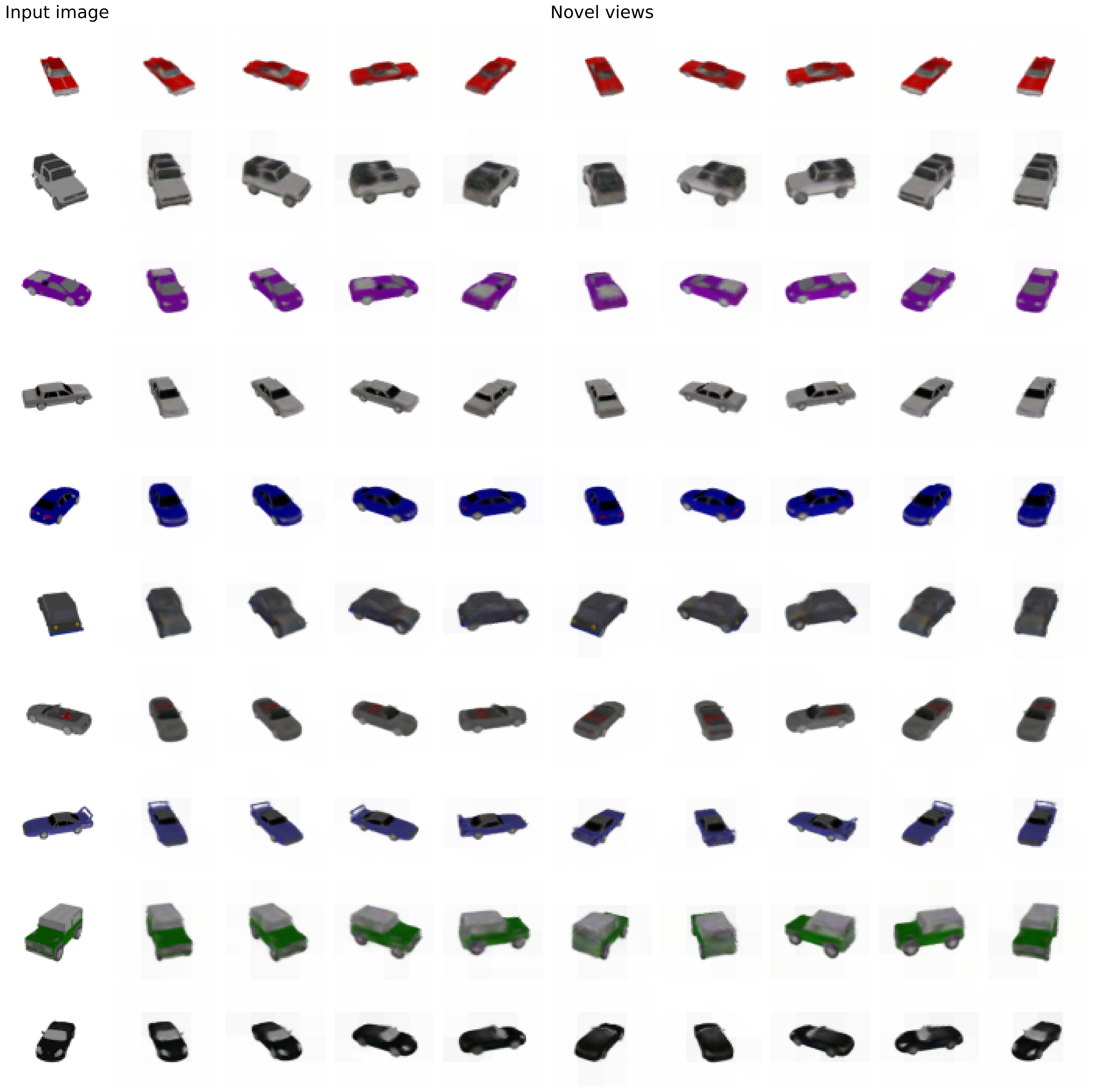
8. Evaluation: novel views from a single image

After training, we run the model on unseen test scenes. For each one, we pick a single source view, predict Gaussians, and render from a grid of held-out target cameras.

@torch.no_grad()
def render_novel_view_grid(model, gt_pixels, c2ws, intrinsics, H, W, znear, zfar,
                           device, save_path="splatter_image.png", num_test_scenes=10):

    novel_view_indices = [1, 2, 4, 7, 10, 13, 16, 19, 22, 23]
    ncols = len(novel_view_indices)
    fig, axes = plt.subplots(num_test_scenes, ncols,
                             figsize=(2.2 * ncols, 2.2 * num_test_scenes), dpi=300)

    for scene_idx in range(num_test_scenes):
        scene_imgs  = gt_pixels[scene_idx]
        scene_c2ws  = c2ws[scene_idx]
        scene_intr  = intrinsics[scene_idx]

        src_view_idx = novel_view_indices[scene_idx]
        tgt_view_indices = [v for v in novel_view_indices if v != src_view_idx]

        src_img    = scene_imgs[src_view_idx].permute(2, 0, 1).unsqueeze(0).to(device)
        source_c2w = scene_c2ws[src_view_idx].to(device)
        source_cam = scene_intr[src_view_idx].to(device)

        fx_src, fy_src, cx_src, cy_src = intrinsics_to_fxfycxcy(source_cam, H, W)
        raw = model(src_img)

        pos, color, opacity_raw, sigma = decode_gaussians(
            raw=raw, source_c2w=source_c2w, fx=fx_src, fy=fy_src, cx=cx_src, cy=cy_src,
            znear=znear, zfar=zfar)

        for col_idx, view_idx in enumerate(tgt_view_indices, start=1):
            target_c2w = scene_c2ws[view_idx].to(device)
            target_cam = scene_intr[view_idx].to(device)
            fx_t, fy_t, cx_t, cy_t = intrinsics_to_fxfycxcy(target_cam, H, W)

            pred = render(pos=pos, color=color, opacity_raw=opacity_raw, sigma=sigma,
                          c2w=target_c2w, H=H, W=W, fx=fx_t, fy=fy_t, cx=cx_t, cy=cy_t)
            axes[scene_idx, col_idx].imshow(pred.detach().cpu().numpy().clip(0, 1))
            axes[scene_idx, col_idx].axis("off")

This is the moment of truth. The model has never seen these objects. It only sees one image of each. And yet the predicted Gaussians can be rendered from arbitrary novel viewpoints in plausible-looking ways — all in a single forward pass, no optimization at test time.

What's next

In the next post in this feedforward 3DGS series, we will look at how to predict multiple Gaussians per pixel, so the network can also represent occluded geometry. That single change pushes single-view reconstruction quality dramatically closer to multi-view methods, and it is one of the main directions modern feedforward 3DGS work has taken.

If you want to be notified when that one comes out, subscribe to the newsletter below.

Final thoughts

Splatter Image is a small but striking demonstration of how parameterization shapes what neural networks can learn. The whole feedforward 3DGS pipeline works because:

• Per-pixel Gaussians let a UNet predict 3D structure with familiar spatial inductive biases.
• Each output channel is bounded and physically meaningful, not raw scene coordinates.
• Output-head initialization gives the optimizer a sensible starting point.
• Differentiable rasterization closes the loop — pixel loss, then backprop everything.

There is no per-scene optimization loop. There is no meta-learning. Just a UNet, a clean parameterization, and a renderer.

Full code: github.com/MaximeVandegar/Papers-in-100-Lines-of-Code/Splatter_Image_Ultra_Fast_Single_View_3D_Reconstruction

Learn 3DGS Step-By-Step

Newsletter

Consulting